What Is Negative-Shifted Gradient Descent—When the Useful Estimator Is Not an Endpoint
Paper · alphaXiv · Code · Interactive Research Highlight
We usually define a regularized estimator by an endpoint: write down an objective, solve it in closed form or run an algorithm until it converges, and call the limit the estimator. The computation is treated as a route to that destination.
Negative-shifted gradient descent (NS-GD) starts from a different possibility. What if the statistically useful estimator lies on the path, in a region where no stable endpoint exists?
This is not a metaphor in the head–tail model studied in our paper. The correction that exactly removes implicit head shrinkage can place the signed level at the very spectral location where a negative-ridge endpoint blows up.
Finite time is not an approximation to the endpoint. It creates an estimator that the endpoint cannot represent.
Endpoint thinking is natural—but restrictive
Closed-form and converged estimators remain valuable: they are analyzable, reproducible, and often inexpensive to compute. The habit of identifying the estimator with a stationary solution also reflects a period when optimization was mainly expected to deliver that solution.
Modern iterative computation gives us another design space. Once the whole trajectory is available, there is no statistical reason to assume that its infinite-time limit must be its best point. A stopping time can be a regularization parameter, and a deliberately nonconvergent direction can still pass through a well-controlled estimator.
The distinction is conceptual:
- Endpoint regularization asks which stable objective or inverse we should solve.
- Path regularization asks which finite-time spectral transformation gives the best prediction tradeoff.
NS-GD matters because these two questions have different feasible answers.
The useful correction can sit at the pole
Consider an overparameterized head–tail model. A signal-bearing head has population scale \(\lambda_h\). The tail contains \(d_T\) individually weak directions, each with scale \(\lambda_T\). If \(\gamma_T=d_T/n\), their aggregate sample-space contribution behaves approximately like the scalar floor
The floor stabilizes interpolation, but the head is then recovered only at the attenuated ridgeless level
In the ideal common-spike model, the exact correction uses
Why is this striking? The observed head location is also \(a+\lambda_h\). Thus the useful signed level satisfies \(\nu_\star=\mu_h\): it is placed exactly where the negative-ridge endpoint
has its pole.
A stable negative-ridge endpoint must keep that pole below the entire positive empirical spectrum,
But random-matrix geometry places the Marchenko–Pastur lower edge near
well below \(\nu_\star=a+\lambda_h\). The desired correction is therefore not merely difficult to reach by negative ridge. It lies outside the stable endpoint class, and in the ideal model its target head mode is the endpoint pole itself.
A closed-form inverse is not necessarily a stable solution
There is an important precision here. If \(\nu\) is above \(\widehat\mu_{\min}^{+}\) but does not equal an empirical eigenvalue exactly, one may still be able to write the algebraic expression
on the empirical row space. But this does not make it a stable negative-ridge endpoint. Directions with \(\mu<\nu\) have negative curvature, the quadratic objective is not bounded below along those directions, and gradient dynamics grow instead of converging. Near \(\mu=\nu\), the rational inverse is also arbitrarily sensitive; at equality, it is undefined.
So “the inverse can be written” and “the estimator can be reached as a stable regularized solution” are different statements. Beyond the endpoint wall, the former may hold away from exact poles; the latter does not.
Finite time changes the singularity
The continuous-time idealization of NS-GD has spectral filter
The integral representation reveals the key fact:
The endpoint pole is removable at every finite time. At the common-spike choice \((\nu_\star,t_\star)\),
The finite path therefore cancels the implicit attenuation exactly in the ideal floor model, even though the corresponding endpoint is singular at that same head location.
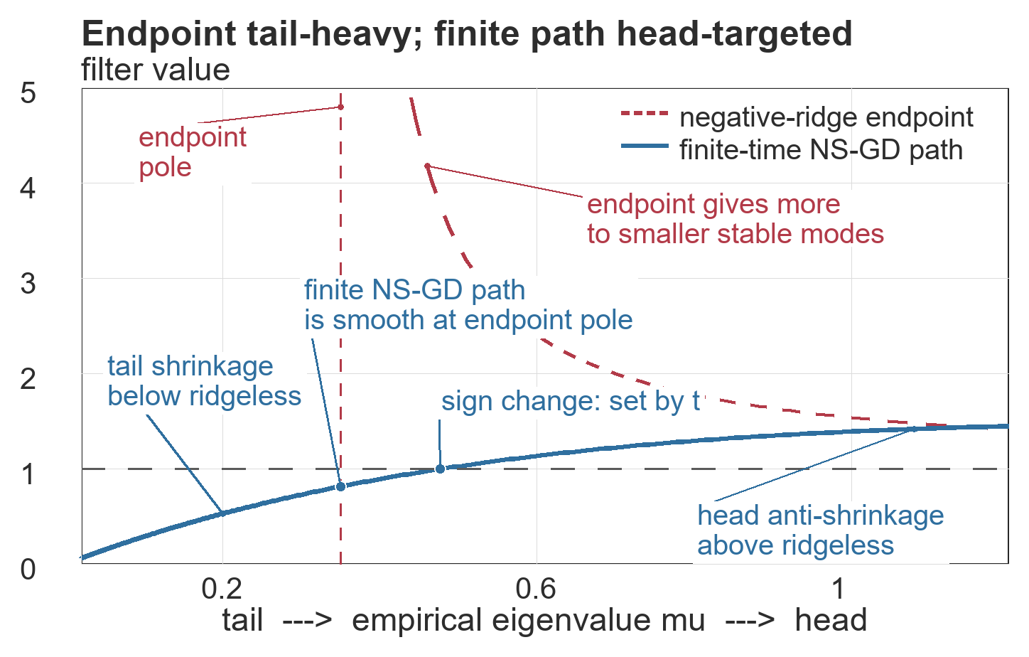
For an interactive version of this filter and a separate illustration of the Marchenko–Pastur barrier, see the Research Highlight.
The path is the statistical object
Once we stop treating iteration as merely a numerical approximation to a closed-form answer, the role of NS-GD becomes clearer. The signed level \(\nu\) chooses a correction scale that a stable endpoint may be unable to access. The stopping time \(t\) limits how long the lower spectrum is exposed to the noncontractive dynamics.
Together, these two parameters create mixed-sign spectral regularization. The sign refers to the displacement from ridgeless regression, \(f_{\nu,t}(\mu)-1\): selected leading modes can be anti-shrunk above one, while lower modes remain below one or exposure-controlled. A single stable negative-ridge endpoint cannot produce this leading-prefix shape; its amplification instead grows toward its lower-spectrum pole.
This does not mean that every unstable trajectory is useful. The recovered-signal gain must exceed the variance and lower-spectrum exposure price. In practice, NS-GD evaluates a finite grid of signed levels and stopping times and uses validation to choose among finite iterates. Discrete NS-GD is the controlled finite-step implementation; the smooth formula above describes its continuous-time geometry.
The larger lesson is that computation can expand the statistical estimator class. Closed-form endpoints are still important, but they need not define its boundary. When the useful correction lies at or beyond an endpoint pole, convergence is not the goal—it is the constraint that must be avoided.
Takeaway
Negative ridge identifies the correct direction of correction, but stable negative-ridge endpoints cannot reach the required magnitude in the regime studied here. Finite-time negative-shifted dynamics can.
The optimization path is not just how we compute the estimator. In this problem, the path is where the estimator exists.
Enjoy Reading This Article?
Here are some more articles you might like to read next: