Shrinkage Is Not a Universal Law

For a concise overview of the paper and its background, see alphaXiv.

One of the most famous lessons in statistics comes from the James–Stein phenomenon: when estimating many noisy quantities, pulling the estimates toward zero can reduce their total error.

That discovery helped make shrinkage a central principle of modern statistics and machine learning. Ridge regression, regularization, weight decay, early stopping, and many Bayesian estimators are all built around a similar intuition:

A slightly biased but less variable estimate can outperform an unbiased one.

This principle is powerful. But the popular slogan it inspired—“when estimates are noisy, shrink them”—is not a universal law.

In overparameterized prediction, sometimes the correct action is the opposite:

Some directions should be expanded rather than shrunk.

The missing part of the classical bias–variance story

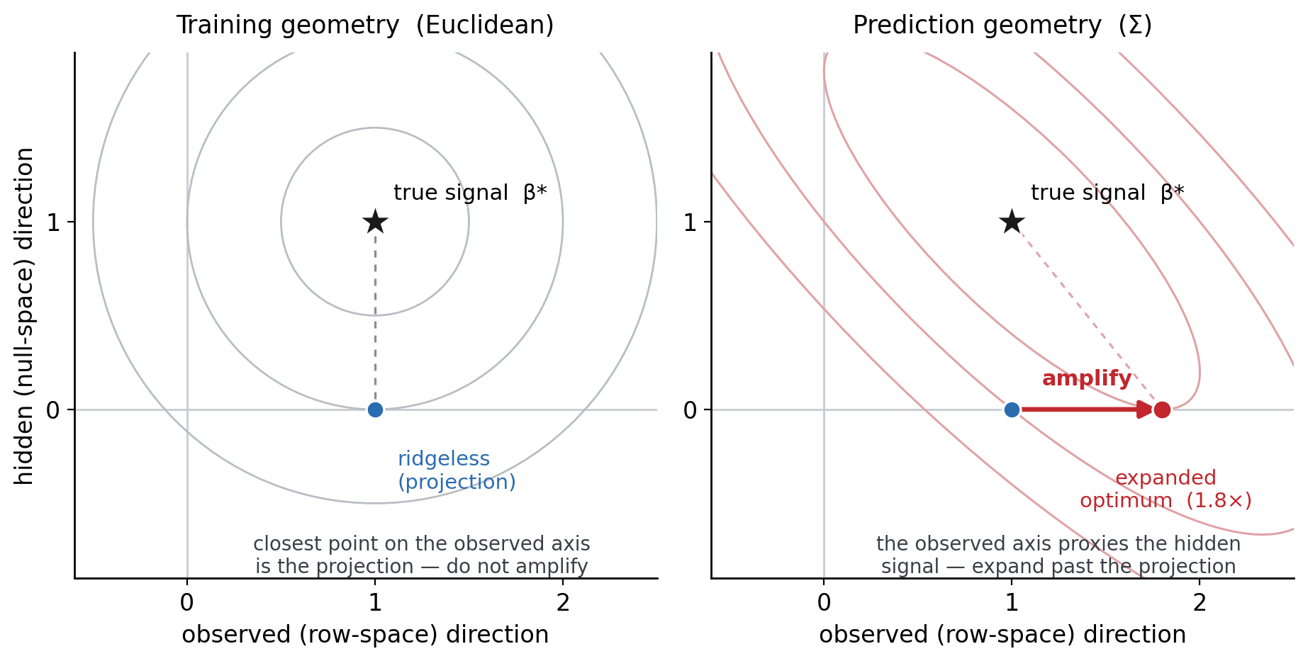
Consider linear regression with more parameters than observations. The training data can identify only the component of the true signal lying in the empirical row space of the design matrix. Another component remains in the empirical null space and is invisible to the training loss.

The minimum-norm, or ridgeless, estimator sets this unobserved component to zero.

In ordinary Euclidean geometry, the empirical row space and null space are orthogonal. This may suggest that increasing a fitted row-space coefficient cannot help recover signal in the null space.

But prediction error is not necessarily measured in Euclidean geometry. It is measured using the population covariance of future predictors.

When that population covariance is anisotropic, two directions that are orthogonal in the training geometry need not be orthogonal for prediction. A direction visible in the training data may therefore act as a proxy for signal hidden in the empirical null space.

Increasing its fitted coefficient can improve test prediction.

Of course, amplification also increases noise. For each direction, this creates a simple competition between two quantities:

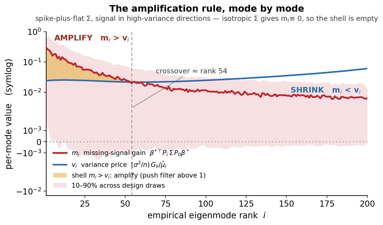
\(m_i\) — the missing-signal gain: how much amplifying the observed coordinate recovers of the hidden null-space signal, measured in the population-covariance geometry.

\(v_i\) — the variance price: the extra estimation noise the same amplification injects.

Our result gives an exact, direction-by-direction rule — amplify exactly when the gain beats the price:

This is not a rejection of the bias–variance tradeoff. It is the bias–variance tradeoff with an important source of bias restored.

When does classical shrinkage return?

In aligned settings, the missing-signal gain vanishes.

For example, if the population covariance is the identity, empirical row-space and null-space directions remain orthogonal for prediction. The gain \(m_i\) is then zero, while amplification still carries a positive variance cost.

The classical shrinkage conclusion is recovered.

Likewise, if risk is measured using the empirical training geometry, the null-space signal contributes nothing to that risk. If the design has full column rank, there is no empirical null-space signal to compensate for.

The classical setting is therefore not wrong. It is a special geometry in which the benefit of anti-shrinkage has been removed.

A broader statistical rule

The general lesson is therefore not:

Always shrink.

Nor is it:

Always anti-shrink.

The more complete rule is:

Shrink when the variance saving exceeds the lost signal. Expand when the missing-signal gain exceeds the variance price.

James–Stein revealed that unbiasedness is not always optimal.

The overparameterized prediction setting reveals a complementary fact: shrinkage itself is not always optimal.

The right decision depends on the geometry of what the data observe, the geometry in which performance is evaluated, and where the signal is located.

Paper: Beyond Negative-Ridge Endpoints: Mixed-Sign Spectral Regularization via Negative-Shifted Gradient Descent.