The Spectrum Was Known to Be Biased. Why Did PCR Keep Inverting It?

For a concise overview of the paper and its background, see alphaXiv.

Principal component regression (PCR) is one of the oldest and simplest forms of spectral regularization. Compute the empirical principal components, keep the leading ones, discard the rest, and perform regression in the retained subspace.

This creates a familiar question:

How many principal components should we keep?

For standard PCR, rank selection determines which empirical directions are retained. Once a direction is retained, however, PCR uses its empirical eigenvalue in the inverse. This distinction matters in high dimensions: when the dimension is comparable to the sample size, empirical eigenvalues need not closely track population spectral scales. Even an identity population covariance produces a dispersed sample spectrum under the Marchenko–Pastur law, while spiked-covariance theory describes systematic distortions of leading sample eigenvalues and eigenvectors.

Covariance estimation has long treated this discrepancy as an estimation problem. The literature includes linear shrinkage, population-spectrum recovery, eigenvector-aware bias correction, and nonlinear eigenvalue shrinkage. These methods differ technically, but share a common premise: empirical covariance eigenvalues should not automatically be used as if they were population eigenvalues.

Standard spectral-cutoff PCR usually addresses a different part of the problem. It changes which directions are inverted, but not the empirical eigenvalues used in the retained inverse weights. This leads to a natural question:

If spectral distortion is worth correcting in covariance estimation, what happens when the same distorted eigenvalues are subsequently inverted in PCR?

Our recent paper on de-floored principal component regression (dPCR) starts from this question.

But PCR is an inverse problem

Here is where something interesting happens.

Suppose a predictive population component has spectral scale \(s_i\), but high-dimensional random design inflates its empirical denominator to approximately

For covariance estimation, seeing an eigenvalue that is too large naturally suggests correcting it downward. But regression uses the eigenvalue in the denominator.

Ordinary PCR effectively applies the inverse weight \(1/(s_i+a)\), so the resulting signal multiplier is approximately

So the same upward spectral distortion that covariance estimation tries to remove becomes downward attenuation of the regression signal after inversion.

Correcting \(s_i+a \longrightarrow s_i\) means changing the regression weight from

In other words:

Shrinking an inflated covariance eigenvalue corresponds to anti-shrinking the associated regression coefficient.

This inversion changes the statistical interpretation completely.

Standard PCR regularizes the support, not the retained denominators

Classical spectral cutoff methods solve instability by changing which singular directions are used.

A retained empirical component receives its ordinary inverse weight \(1/\widehat\mu_i\), while a discarded component receives weight zero. PCR therefore has a binary spectral decision:

What it does not normally ask is whether the retained empirical eigenvalue \(\widehat\mu_i\) itself contains a systematic nuisance component that should be removed before inversion. This distinction is explicit in our paper: ordinary spectral cutoff changes the support of the inverse filter, whereas dPCR changes the denominators within the retained range.

That matters because no rank choice can repair a wrong denominator. If a predictive component is retained, PCR inherits its attenuation. If it is discarded, PCR loses the component entirely. Neither choice produces the correct inverse weight.

When does self-induced regularization become over-regularization?

Suppose the covariance has a predictive head and a very large collection of individually weak tail directions. Write the sample-space Gram matrix schematically as

When the tail has sufficiently high effective dimension, \(K_T \approx a\,I_n\), where

The tail therefore creates a nearly scalar spectral floor underneath the predictive head, and a head component with clean scale \(s_i\) appears roughly at \(s_i+a\).

If \(a \ll s_i\), the attenuation \(s_i/(s_i+a)\) is negligible. This is effectively the strong-signal regime. The floor may be visible spectrally but does not matter at first order for prediction. This helps explain why the correction is absent from much traditional theory: assumptions that make the signal sufficiently strong also make the floor-induced bias asymptotically irrelevant.

But consider instead the matched regime \(a \asymp s_i\). Now \(s_i/(s_i+a)\) is bounded away from one. The implicit shrinkage is no longer a small perturbation—it creates first-order prediction bias.

The question becomes:

Can we remove this floor without paying an equally large variance price?

First spectral mass creates the bias; squared spectral mass determines the price

This is the key structural result of the paper.

Define

The spectral floor is generated by the first tail mass, \(a = T_1/n\), so its squared attenuation effect is governed by \(T_1^2\). But the clean prediction cost associated with the tail after correction is controlled by the squared tail mass \(T_2\). Our exact risk decomposition separates precisely these two quantities: first spectral mass controls denominator inflation, while squared spectral mass controls the clean prediction cost of correction.

This opens a regime that is easy to miss if one thinks only in terms of "large" or "small" tails. A tail can simultaneously have \(T_1\) large and \(T_2\) relatively small. The relevant condition is

Equivalently, its effective dimension \(d_{\mathrm{eff}} = T_1^2/T_2\) satisfies \(d_{\mathrm{eff}} \gg n\). This is the central asymmetry:

Many individually weak directions add coherently to create a large common spectral floor, but their prediction cost accumulates only through squared spectral mass.

The floor can therefore be large enough to matter while remaining cheap to remove.

De-floored PCR

dPCR makes the simplest possible correction. Where ordinary PCR uses \(1/\widehat\mu_i\) on retained components, dPCR uses

where \(a_0\) estimates the spectral floor. Rank and floor correction play different roles:

• the rank determines which empirical directions are trusted;
• the floor correction determines how strongly the trusted directions should be inverted.

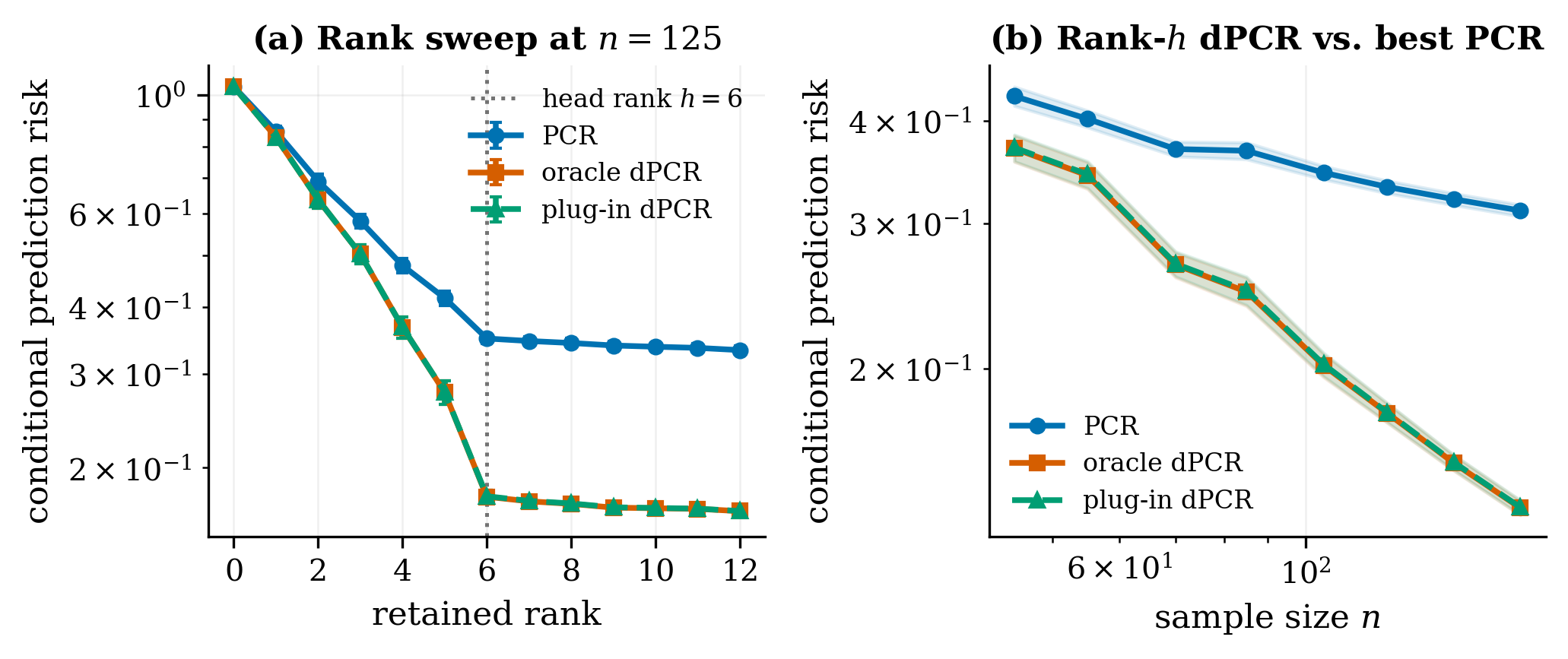
In the sharp-floor regime, the floor can be estimated from the same empirical spectrum using the lower spectral cluster. Our theory shows that this plug-in correction attains the oracle dPCR rate at a prespecified retained rank. More importantly, in the matched sharp-floor asymptotic regime, the prediction risk of dPCR becomes negligible relative to the best ordinary PCR risk over all possible ranks. This targets the sharp-floor regime specifically: in the ordinary proportional Marchenko–Pastur bulk, where the spectrum has persistent relative width, a single scalar correction is not enough.

So the gain cannot be explained by better rank selection.

The missing regularization axis is denominator correction.

A familiar phenomenon viewed through an inverse

This is perhaps the most interesting part of the story. Random-matrix theory and covariance estimation both told us the empirical spectrum is distorted and worth correcting.

PCR nevertheless continued to use those eigenvalues primarily through a spectral cutoff: retain \(1/\widehat\mu_i\), or replace it by zero.

Our result suggests another possibility:

Before inverting an empirical eigenvalue, ask whether part of it is an endogenous spectral floor that should not be there.

The same spectral inflation that looks like a covariance-estimation error becomes a coefficient attenuation after inversion. And the same high-dimensional tail that looks like beneficial implicit regularization in one regime can become removable over-regularization in another.

That leads to a broader statistical principle:

A regularization effect should not be judged only by how much variance it removes. We should also ask what systematic bias it creates, whether that bias is identifiable, and whether removing it costs less than leaving it in place.

For dPCR, that comparison has an unusually clean form:

The spectral floor was not unknown. What was missing was the regime in which, after inversion, it becomes a first-order but cheaply removable prediction bias.

Paper: De-floored Principal Component Regression: When Rank Selection Alone Is Insufficient for Prediction.